

Material Models for HSLA
Material modelling for high-strength low-alloy steels used in demanding automotive, infrastructure and heavy-engineering applications.
Written by
Bijish Babu
Published
Topics
- FEM
- Manufacturing
- MatMod
HSLA Steels provide better strength with respect to corrosion properties. Therefore they are widely used in applications related to automobiles, cranes, bridges, roller-coasters etc. However the deformation mechanisms during the processing of this alloy is also complex as it involves varying phases, different mechanisms like recovery, recrystallization, etc, as shown in the figure below.
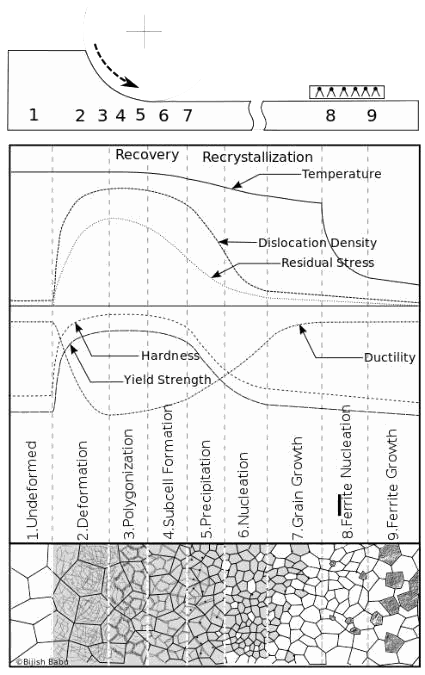
A constitutive model, which has to take into account of the above phenomena, should be based on the physics of material behaviour. Macroscopic plasticity effects and properties of dislocations are related. Plastic strain is associated to motion of dislocations and hardening / softening is associated to interaction of dislocations. The proposed model has capability to connect to the microstructure of the material. The basic formulation is explained in an earlier post or in Babu and Lindgren (2013).
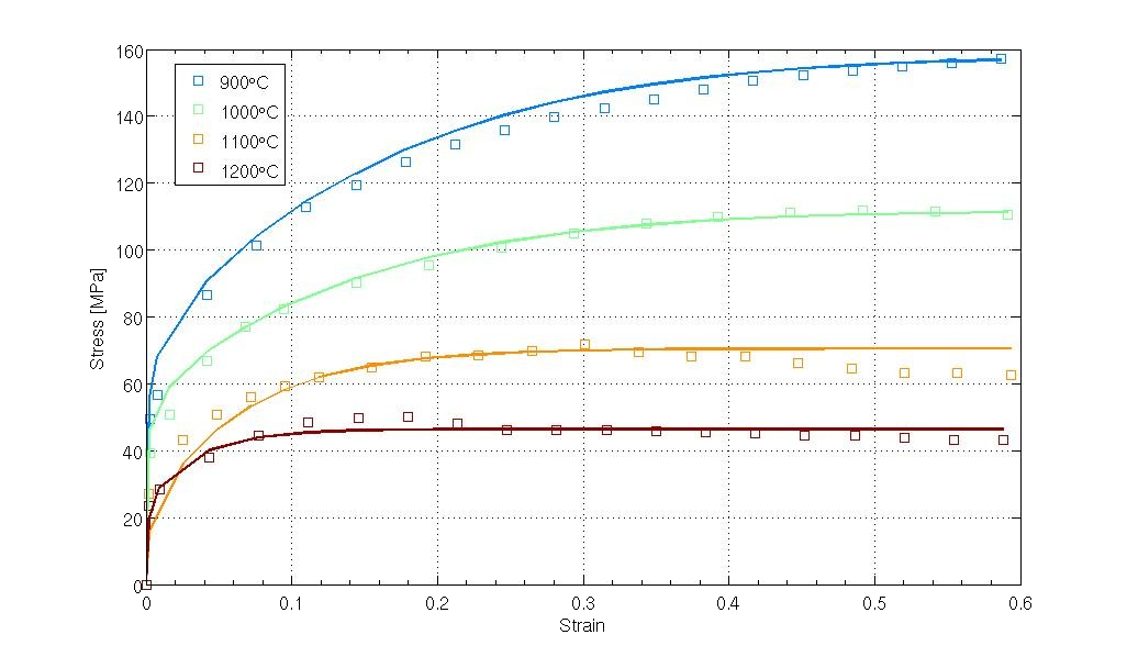
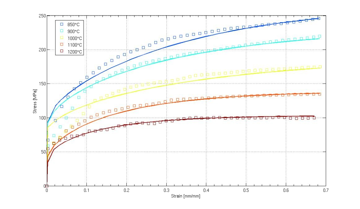
Compression tests performed at the nominal temperatures between 850°C and 1200°C and strain rates from 0.01s-1 to 10.0s-1 taken from Bäcke (2009) for C-Mn Steel were used to calibrate the model. The calibrated model (continuous lines) along with the measurement data (points) is given in the figures below.
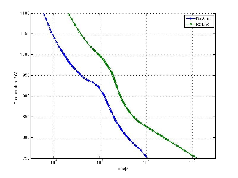
The Recrystallization kinetics is modeled by using an Avirami type equation. The parameters for this model are found from literature using the start time and end time of recrystallization taken from Gladman (1997). This data along with the fitted model for start and stop is given in the figure below.
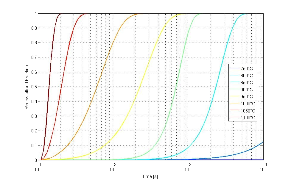
The predictions of the model during iso-thermal hold are given in the figure below. This is computed by instantly cooling from 1200°C and holding at specified temperature for a certain time.
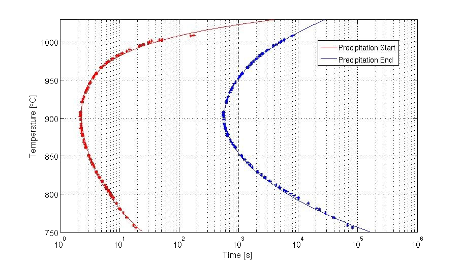
If small quantities of Nb and/or Ti are added to C-Mn steel, Nitrides and Carbides are formed and they can contribute to additional strengthening of the material. The precipitation kinetics can be modeled in the same fashion as that of recrystallization. The data for precipitation start and finish is taken from Gladman (1997). The model fitted to this data along with the original data is given in figure below.
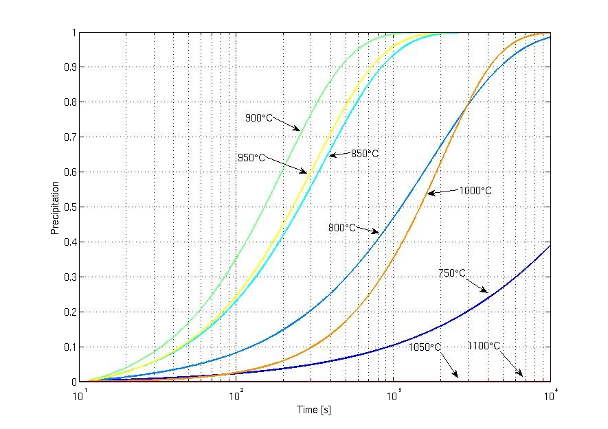
The predictions of the model for precipitation are given in the figure below. This is computed by instantly cooling the material from 1200°C and holding at the specified temperature for a certain time.
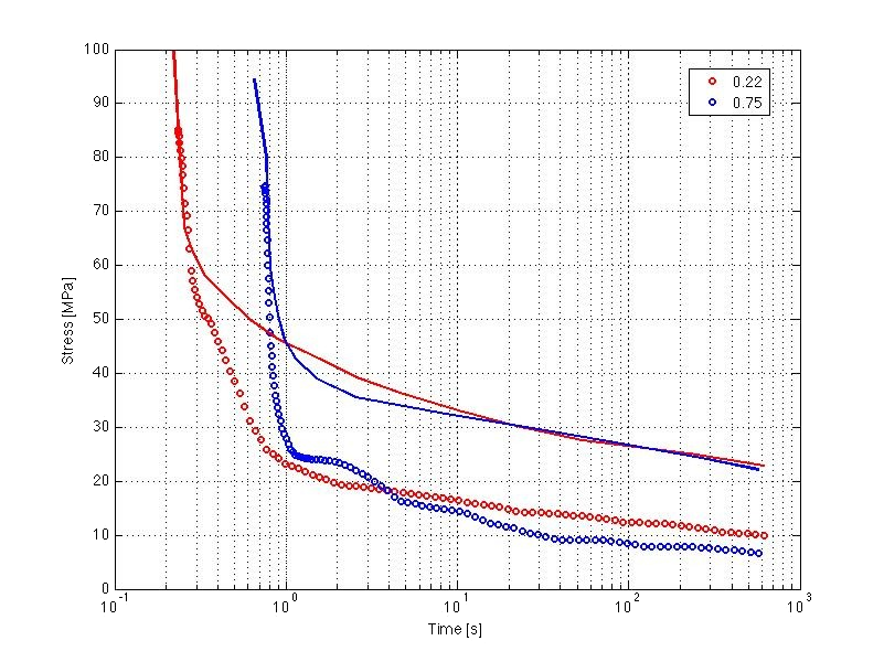
In order to validate the model, stress relaxation tests were performed at 1050°C and at two different strains (22% and 75%) see figure below. The points denote measurements and lines denote predictions of the model. The model for stress relaxation during recrystallization is able to replicate the exponential drop of strength. The difference between the measurement and prediction of 20MPa can be attributed to the fact that the model was calibrated with another grade of steel than tested below.
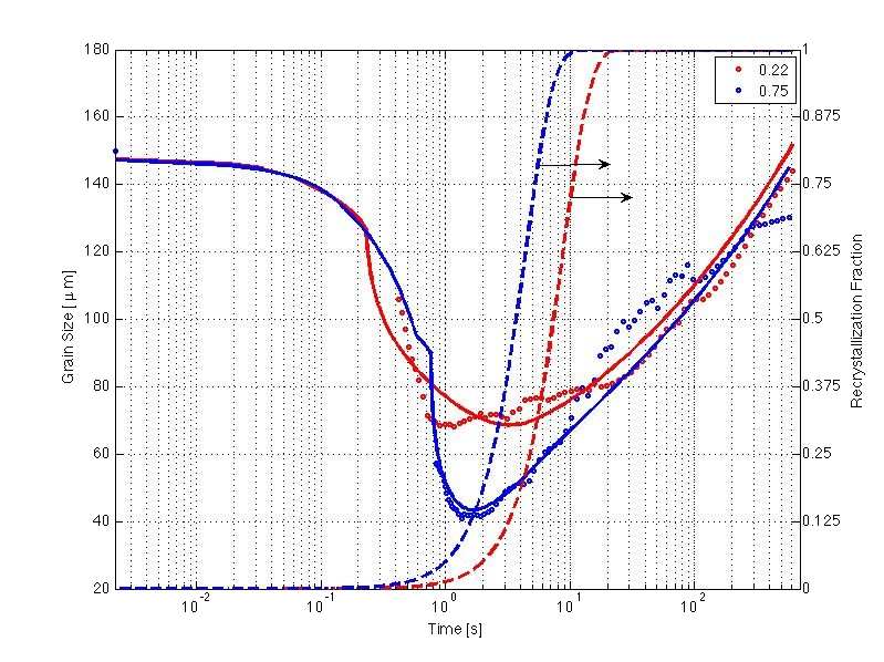
During these tests, measurement of grain size was also performed using laser ultrasonic technique and is given in figure below. The points denote measurements and lines denote predictions of the model. The model for average grain size evolution consists of two models: one for grain size reduction during recrystallization and other for grain growth. These models were able to capture the phenomenon very closely. Also the computed fraction recrystallized is also shown below as dotted lines.
A calibrated thermo-mechanical-microstructural model for HSLA steel to be used in simulations of involving arbitrary thermo-mechanical loading is presented here. The internal state variable approach followed here to compute the evolution of material state could be implemented in any standard finite element software.
References
- B. Babu, L.-E. Lindgren. (2013). “Dislocation density based model for plastic deformation and globlarization of Ti–6Al–4V”Int. J. Plast., 50 (2013), pp. 94–108
- Bäcke, L. (2009). “Modeling the Microstructural Evolution during Hot Deformation of Microalloyed Steels”. (Ph.D. Thesis). Stockholm: KTH. ISBN: 978-91-7415-267-8
- Gladman, T., (1997). “Precipitation behavior of particle coarsening”. In: The Physical Metallurgy of Microalloyed Steels, London: Institute of Materials.
Originally published by Bijish Babu on LinkedIn: Material model for HSLA Steels