How to Calibrate Material Models?
Introduction
To perform Finite Element (FE) simulations, the material behavior needs to be modeled numerically. A wide range of models exist in the literature (see table at the end), capable of capturing different aspects of metal plasticity; strain rate and temperature dependence. Most of the commercial FE software has a variety of material models implemented in its library. Therefore, the analyst should choose the constitutive models judiciously depending on the requirements to perform a “sufficiently” accurate simulation. Many of these models are based on empirical observations, except a few founded on the physics of deformation mechanisms. Physics-based models are comparatively complex, and their calibration for a particular material is not trivial.
Calibration of Material Models
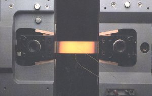
Calibration of model parameters to material data is performed by using inverse theory. Inverse problems are a large class of problems usually found when looking for the causes of an observed physical phenomenon. They can generally be formulated according to equation σ = F(p), where p is the set of parameters to be determined. Two problems are called inverse to each other if the formulation of one problem involves the solution of the other one. These problems are common in science and technology; measurement of temperature by recording the electric potential and measurement of strain by recording the electrical resistivity.
If a problem has a unique and stable solution, it is called well-posed. Commonly, inverse problems are not well-posed because the stability criterion is not satisfied. Nonlinear inverse problems can also be written according to the equation above. But here, F is a nonlinear operator and cannot be separated to represent a linear mapping of the model parameters. Examples of these problems include weather prediction, medical imaging, non-destructive testing, etc.
The parameters for a flow stress model can be identified by comparing the flow strength measurement with computed flow stress. The experimental results from a compression or tension test machine include stress, strain, time, and temperature denoted by σ, ε, t and T respectively for each experiment. The model for flow stress can be written as σy = F(ε, ε̊, T, p (ε, ε̊, T)). The parameters p can be calibrated by matching the measurements with the model. Therefore, the cost function can be formulated as
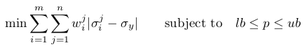
where 0 ≤ wi ≤ 1 is the weight factor, n is the number of experiments, m is the number of measurement points for each measurement, and ub, lb are the upper and lower bounds. The cost function is dependent on the experiment and flow-strength model considered here.
Material Modeling Platform
A platform for calibration has been developed, which has several additional purposes. It consists of three modules; pre-processor, optimizer, and post-processor. Though this post describes the tool in the context of flow stress models, it is not limited. This software has been used to calibrate many other models like Fröhlich’s B-H relation, TTT curves, Bouc-Wen, etc. This software is used as a database for storing raw material data from tests, processed data after smoothing and reduction, pedigree information, ownership, etc.
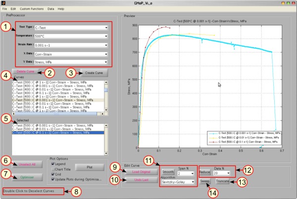
Preprocessor
The pre-processor can import and process measurement data (time, strain, stress, temperature, etc.). Smoothing, reducing, and truncating the data are the most commonly used features. The original and processed data are saved in a database together with existing model parameters.
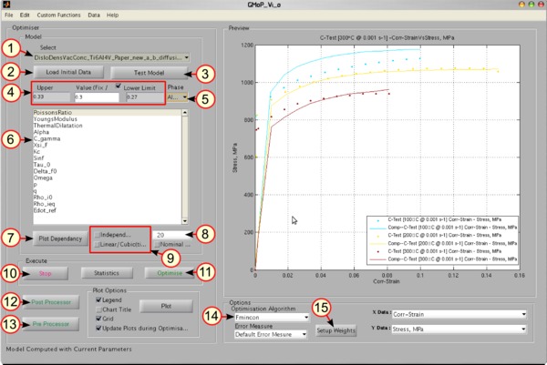
Optimizer
The optimizer module makes it possible to interact with the calibration process. Here, the parameters can be fixed or free for calibration, and the upper and lower bounds of each parameter can be defined. The parameter set used in the calibration can be changed during the calibration process.
Common Flow-Stress (Material) Models
The most commonly used approach to model isotropic plasticity is von Mises or J2 plasticity. According to f(σy, J2 ), the yield surface can be formulated, where σy is the yield strength written as an equation and J2 is the second invariant of stress. The radial return algorithm is widely used to integrate isotropic J2 plasticity. Engineering or empirical equations for σy are developed utilizing fitting parameters of equations with experimental data ignoring the physical processes causing the observed behavior. This kind of modeling approach is more common in engineering applications and therefore got the name. A subset of models implemented within the platform is given in table 1.
This software has been used in calibration of more advanced and complex material models described in the posts
This software platform is used in the calibration of the models and offered as a packaged service for testing and calibration from Aerobase.